Xarray and working with NetCDF data

Xarray focuses on providing a better implementation of multi-dimensional arrays than Numpy. Real world multi-dimensional data cannot be easily represented by just raw numbers, which the Numpy version of arrays are. For example, weather datasets contain several variables (like air temperature, specific humidity, wind speed), coordinate variables (like latitude and longitude), and dimensions.

This is how a typical weather dataset structure looks like:

Data Structures in xarray:

There are two main data structures provided by xarray –

• DataArray
• Dataset

DataArray class implements multi-dimensional arrays with dimension names, coordinates, and attributes linked to them.

Dataset is a combination of multiple xarray DataArrays. It is a dictionary like container which maps one variable to each DataArray it holds.

Below is an example of a dataset that holds the variable tas (near surface air temperature).

We can breakdown this output into the descriptions of –

• Dimensions – time, bands, latitude, longitude along with their lengths
• Coordinates mapped with dimensions mentioned in parentheses (A dimension may or may not have a mapped coordinate). Coordinates themselves are dictionary like container that map coordinate names to values. For example:

Here, time is the coordinate name, (time) is the dimension name to which it is attached, datetime64[ns] is the datatype of individual values of the time coordinate, the values in the array are the individual coordinate values and can be visualized as ticks of an axis of a graph.[There are also non dimension coordinates, but we will not get into the details of that as of now.]

• Data variables which are themselves DataArrays, along with their dimensions in parentheses. These dimensions are a subset of the complete list of dimensions listed at the beginning at the dataset level.
• Attributes

We can try to access a single array out of this dataset. Since the main variable of importance here is ‘tas’, we can try selecting that:

Working with NetCDF data

Downloading, extracting, reading the data into xarray dataset

Below code snippet downloads CMIP6 dataset, from Copernicus climate datastore. The region selected below broadly encompasses the geographical region of India, though not with 100% accuracy:

This downloads one file for each variable listed in the vars list. The downloaded files are zipped. Below code snippet can be used to unzip the files

Reading the downloaded NetCDF files into xarray datasets:

Exploring one of the datasets:

Selecting one variable of the dataset individually, which itself is a DataArray

Selecting data through different kinds of indexing:

Using .sel() and .isel() to index data from tas variable within the dataset ds_cmip6_tas.

In the above example, position-based indexing has been used. We can make the same selection by passing the label of the first longitude using the .sel() method.

Selecting using the first label of longitude

Another useful functionality is the ‘nearest’ method. If we do not know the exact label of a coordinate, we can use the approximate value in conjunction with the nearest method.

We can also select a value if we know the coordinate labels against more than one dimensions

Use of masking through ‘.where()’

All the values lying outside the mask will be converted to nan.

Visualizing NetCDF data

Plotting temperature difference between two dates

Plotting aggregations

Plotting aggregations over groups

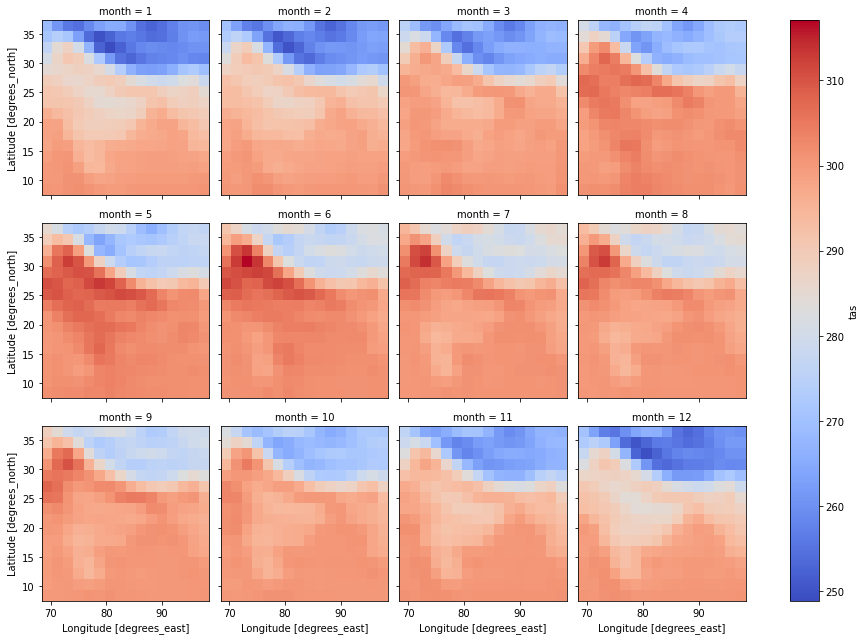
Below is the plot showing mean temperature of each month throughout all years. This is a two dimensional data.

Below plot shows median values for each month of all the years. These median values are calculated over the dimensions – latitude and longitude. Thus, the final plotted data is one dimensional.