Predicting House prices in Ames - Using Regression Techniques
How often, we ponder what is the price to pay for a house that we intend to buy !
Well, I am certain this question has crossed our lives sometime or the other when we made such a big investment in our lives. Would it not be great to be able to predict within reasonable limits (+/- 2% error).
Well, we are possibly heading towards that era where decisions are data-driven. Does that mean everything will be solely formula based? The answer is certainly No ! A part of human life will always be perception driven. You might just like the front design and be willing to pay a premium or you might be desperate to get a roof over your head. Such types of human frailties can never be controlled by an Algorithm ! But leaving that part, you still would like a justifiable price for the investment you are about to make
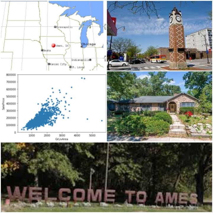
So let us look at a situation ! We have price information for 1460 houses with 79 parameters (or features) and the price. Can we predict the prices for a different set of houses in the same city? This is a problem posted in Kaggle and I am trying to solve this situation
More than 4750 participants have tried to solve this problem. Mine is certainly not the best ! However, my predicted price using algorithmic combination puts me in the top 15%
Salient features of my solution are as below.
- I used Visualization techniques in the Exploratory Data Analysis (EDA) stage to present the data in a concise manner so that a person can capture a good view of the data with very little scrolling. This give a good perspective or bird-eye view of the data
- In the Feature Engineering stage, I used a lot of generic techniques to fill the missing values. Very little 'Hard-coding' has been used. This will ensure that the notebook can be used on a different set of data whose data elements might be the same but the characteristics of the data is very different.
- Lastly, in the model-fitting stage, I have used a weighted average of the models that are used. Since, the blended model provided a better RMSE score, I used that in the final prediction of the price.
1. Exploratory Data Analysis (EDA)
First , let us peep into the price distribution visually by plotting the same into a distribution plot.
1.1 Target Attribute (SalePrice) Observation

As we see, the data is skewed towards the right; in other words the distribution has a tail towards the right. Probing mathematically, the skewness of the data is 1.88 and the kurtosis is 6.54. We shall see later how to transform the data to make it shift towards "Normal"
1.2 Features Observation
A feature will be either Continuous (can take any value e.g PlotSize can be any value in Sq. Ft) or can be Categorical (take discrete values e.g CentralAirConditioning can be "Yes" or "No")
In a concise plot, let us view the relationship between the price and each of the Numeric attributes using scatter-plots.


Let us visualize the Categorical attributes using box-plot graphs

Observations
- LotShape - Has a lot of overlap across two categories.
- LandContour - Has a lot of overlap across 4 categories
- LotConfig - Has a lot of overlap
- LandSlope - Has a lot of overlap
- BsmtFinType1 and BsmtFinType2 have lot of overlaps
- Functional has overlaps across 7 categories
Categorical values having overlap generally cause undue influence on the Algorithms. These are potential features which can be dropped during the Feature Engineering stage
2. Feature Engineering
As part of the Feature Engineering, we need to carry out steps to make the data ready for feeding into the Algorithm. This will be based on the Observations made in the EDA step.
Feature Engineering will involve :
- Removing Features that do not seem to add value, rather might make the Algorithm pick up the noise.
- Removing Outliers .
- Finding out NaN (Null) values and see how to update them without distorting the sets.
- Fixing Skewness of the data
Let us re-look at the Target once more i.e the SalePrice. We noticed that it had a tail towards the right or in other words it had a positive skew of 1.88.
Most models do not perform well if the data-distribution is not normal. So we apply log(1+x) transformation on SalePrice. Let us call this new feature TranSalePrice. How about looking at the SalePrice and TranSalePrice side-by-side?

The above looks more in closer range. So how does the transformed Sale price looks in a distribution plot. Again, let us see them side-by-side.

The transformed Sale Price shows a better distribution and is closer to what is termed as Normal distribution. The tail on the right side is now reduced
2.2 - Work on the Missing features
The ground reality is that no data-set supplied will ever be "Complete". Missing data will hinder the Algorithms to work correctly and will introduce noise. During Real-life data handling, intuition is needed to handle the missing data. The simplest strategy could be to drop the rows/columns. But this will mean loss of data and in the current set of 1460 data samples, it will be a loss to the Algorithm which needs input data to train itself. Rather, we should explore options to fill these missing features with some value that will not disturb the distribution.
As a first step, let is see the extend of missing data graphically

Well, as we see, about five features have "tall poles" in the graph. About 96% of sample data have PoolQC (Pool Quality) missing. Now, as per the data description file, NaN in this field means the House does not have a Swimming Pool. So we update this attribute as "None" for the missing values. Same logic holds for features like MiscFeature, Alley, Fence and FireplaceQC
LotFrontage - is a Continuous Feature. As per Data Description, it is the Linear feet of street connected to property It will be tempting to assign the mean value of the dataset to this feature with the missing values. However, a better way is to find the Median of each Neighborhood and assign the same to the missing rows based on Neighborhood. The assumption being that the LotFrontage will be similar within a Neighborhood.
Electrical, Functional, Utilities, SaleType, KitchenQual

If we look at the distribution, then we find that each of the five features, we have a very small number of NaNs(marked in Yellow). The best solution in this case will be to replace the missing rows with the "Mode" value of distribution.
MSZoning: Identifies the general zoning classification of the sale. A - Agriculture C - Commercial FV - Floating Village Residential I - Industrial RH - Residential High Density RL - Residential Low Density RP - Residential Low Density RM - Residential Medium Density
There is no easy way to default this. The best approximation is to take the Mode of each Neighborhood. This is not a perfect logic, but the this will ensure that for a particular Neighborhood; if it is primarily Residential, then the default will be Residential, if it is primarily Commercial then the default will be Commercial and so on.
2.2 Dealing with Skewed data
Skewed data introduces Noise in the Algorithms. Hence it is necessary to reduce the skewness of data. Let us visualize the skewness first. Skewness is measured fro the Numerical Features

Found that there are 26 Features that have a Skewness above 0.5. Let us reduce skewness by using the Box Cox transformation. Post the transformation, we could reduce the number of skewed Features to 16.
Created a few Additional Features like TotalBathrooms = Sum of all the bathrooms across floors, TotalSquareFeet = Sum of areas of all the floors
Dropped some of the features like Utilities, PoolQc and Street. These features had extreme bias towards one of the Categorical values. The Algorithm will be misled by the distribution
Pearson Correlation - Pearson Correlation gives us a measure of how the Features are inter-related among each others and especially with the Target (i.e SalePrice). A visual representation in the form of Heat-Map is given below. Higher value means greater correlation

Finally, as a last step of Feature Engineering , I did the One-hot encoding to convert the Categorical Features into columns.
3.0 Setting up the Models
For the Regression , I have chosen the following: 1.Light Gradient Boosting Regressor, 2. XGBoost , 3. Ridge , 4. Support Vector , 5. Gradient Booster and 5. Random Forest . And finally used a stacked Regressor to run over the above six Regressors.
I have also used a 4-fold cross-validation on the training data-set to remove bias and get an average score.
From the above step, I have calculated the mean and deviation of each regressors.

It does show that Ridge scored the best in Mean but LightGBM has the least Std Deviation. In terms of computation time, SVM was fastest, taking less than a minute while GradientBooster took about 12 minutes. This is a relative comparison. The time would have been more had the training data-set increased in size or if I had chosen to increase the number of Folds.
All the models were made to fit the data-set.
Also, a blended model was created with all the above models including the stacked Regressor. For the blended model, I chose a weighted score for each based on the Mean and Std Deviation.
Let us now plot the scoring pattern of the different Regressors alongside the Blended model.

The lower the better! We see that Blended model scored way better than the individual regressors.
8.0 Predict the Sale Price of the Test-set
With the models set and test-data prepared, now it is the time to make the prediction of the price for the property for which the price is not provided.
The predicted TranSalePrice and the SalePrice (derived by doing an inverse-transform on the TranSalePrice) we get the predicted price of the properties.
Finally, the predicted price is as below.

Thus, using a combination of Mathematical, logical step and then using computational powers of the Regression Algorithms, we are able to make a prediction of the price.
Now the big question could be "What is the actual Price?". Well ! That is known only to Kaggle and not revealed publicly. However, they score the predicted SalePrice that the participants submit. Based on my submitted forecast, I received a score of 0.11931. That gives me a position of 680 out of 4753. The top 40 participants have a score of 5-Zeros ie. 0.00000.
So, still a lot to learn and improve !